Summary

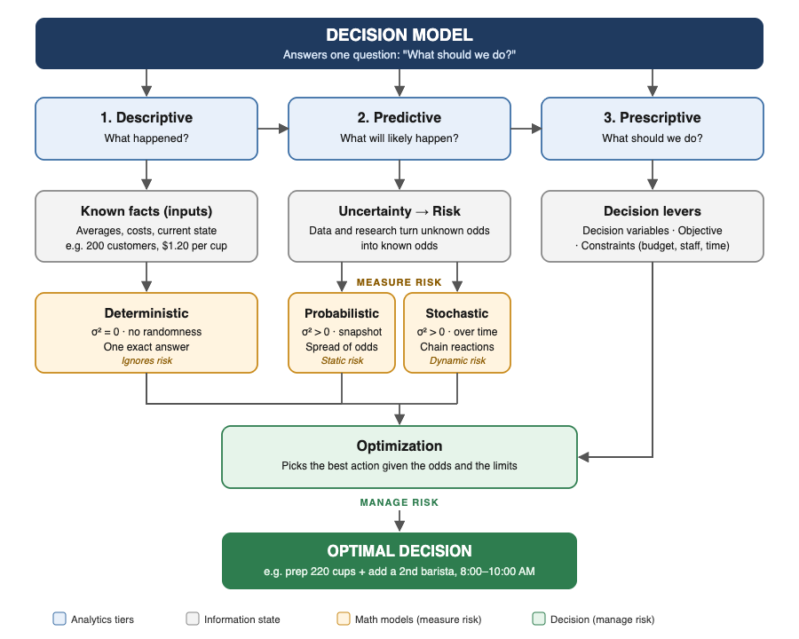
Decision Pipeline: A decision model is a mathematical translation of a business problem, used to evaluate trade-offs and guide action.

Three analytics models: Descriptive (what happened), Predictive (what will likely happen), Prescriptive (what should we do). A decision model uses the first two to produce the third.

Uncertainty vs. risk: Uncertainty means the distribution is unknown, so you reduce it with data and research. Risk means the distribution is known, so you mitigate it with hedges, buffers, and constraints.

Modelled, Measured and Quantified?:

Deterministic : fixed inputs give one exact output.

Probabilistic ( $\sigma^2 > 0$ ): a distribution of outcomes for a single snapshot.

Stochastic ( $\sigma^2 > 0$ over $t \in T)$ : random events unfolding over time, where each step depends on the last.

How is this applied In practice: Descriptive analytics summarises past observed data;. Predictive supplies the odds. Prescriptive applies business constraints and optimizes the decision.

Math reference

Decision Pipeline

A decision model is a formal framework that converts uncertainty into quantified risk and computes the optimal action, under the model’s assumptions and the business’s constraints, so leaders can see the trade-offs and make better-informed choices.

Background uncertainty sampling noise, data latency, measurement error and other errors exist across all modelling domains. While descriptive and predictive models inform decisions by summarising the past or forecasting the future, only Prescriptive models explicitly solve for the optimal choice by evaluating trade-offs across decision variables. Deterministic models simplify this by using fixed point estimates, whereas stochastic models represent uncertainty directly through probability distributions.

1. The Three Analytics Models

Model Type	Conceptual Question	Focus & Techniques	Real-World Healthcare Example
Descriptive	What happened?	Summarizes past data using dashboards, KPIs, and aggregation metrics.	An ICU dashboard tracks that the readmission rate was 18% over the past quarter.
Predictive	What is likely to happen next?	Identifies trends and estimates probabilities using regression and machine learning.	A logistic regression model flags high-risk patients with a ≥70% probability of readmission based on vitals, age, and lab results.
Prescriptive	What is the best action to take?	Recommends optimal decisions using simulation and optimization algorithms.	A decision-support algorithm automatically schedules a 48-hour post-discharge check-in and adjusts dosages to prevent relapse.

2. Uncertainty vs. Risk as a Concept

Uncertainty (Unknown Distribution): Outcomes or their probabilities cannot be reliably quantified (e.g., an unstudied patient cohort).
- Action: Reduce via data collection and research.
Risk (Imperfect Data or Known Distribution): Outcomes carry measurable consequences with estimable probabilities (e.g., historical failure rates).
- Action: Mitigate via hedging, buffers, and decision constraints

Decision model	Where the Uncertainty & Risk comes from	How the model treats it
Descriptive	Sampling error, measurement error, missing or biased data	Often reported as a single number, so it is treated as exact (deterministic). Better practice shows a confidence interval.
Predictive	Unknown future plus imperfect data	Represented explicitly with probabilities (probabilistic or stochastic).
Prescriptive	Everything upstream, plus the chance the model itself is wrong	Manages it with buffers, hedges, and constraints.

3. How Risk is Modelled, Measured and Quantified?

1. Deterministic
   Inputs: Set values ────────► Output: Exact single number (e.g., exactly 200 customers)
   [Assume No chance, no uncertainty]

2. Probabilistic
   Inputs: Distribution ──────► Output: Spread of possibilities for a snapshot in time
   [Static risk]                 (e.g., 95% chance of 150–250 customers tomorrow)

3. Stochastic
   Inputs: Random steps ──────► Output: Path unfolding over time
   [Dynamic uncertainty]         (e.g., hour-by-hour arrivals where morning delays ripple into the noon rush)

3.1 Deterministic (Assumption No Risk)

What it assumes: The world is perfectly predictable. Zero variance $(\sigma^2 = 0)$ .
How it works: $y = f(x).$
Coffee shop math: “Every sunny weekday averages 200 customers. Tomorrow is a sunny weekday, so tomorrow we will have exactly 200 customers.”
Best used for: Simple baseline estimates, cost accounting, or formulas with strict fixed relationships.

3.2 Probabilistic (Static Odds)

What it assumes: The world is random, but we only predict a single, overall outcome (not how it unfolds hour by hour). Variance is greater than zero $(\sigma^2 > 0)$ .
How it works: $Y \sim P(Y \mid X)$ .
Coffee shop math: “Based on historical weather and weekday data, tomorrow’s total traffic follows a normal curve: Mean = 200, Standard Deviation = 25. There is a ~95% probability that traffic falls between 150 and 250 customers (mean ± 2σ).”
Best used for: Setting daily inventory, staffing buffers, or calculating budget risk.

3.3 Stochastic (Chain Reaction Over Time)

What it assumes: Randomness unfolds sequentially over time ( $t \in T$ ), and what happens at 8:00 AM affects what happens at 9:00 AM.
How it works: $\{X_t\}_{t \in T},$ where the state at step t+1 depends on the state at step t (the Markov case).
Coffee shop math: “Customers arrive randomly, on average every 30 seconds. If a sudden surge hits at 8:15 AM, the barista queue grows. Long lines cause 20% of later walk-ins to abandon the queue, shifting demand to 10:00 AM.”
Best used for: Queue simulation, supply chain backlogs, ICU patient flows, and stock trading paths.

Comparison Cheat Sheet

Question	Deterministic	Probabilistic	Stochastic
Is there randomness?	No	Yes $(σ^{2} > 0)$	Yes $(σ^{2} > 0)$
Does time matter?	No	No (one overall summary)	Yes (step-by-step sequence)
Output format	A single number	A probability distribution	A simulated timeline/path
Analogy	Reading a fixed train timetable	Checking the probability of rain tomorrow	Simulating bumper-to-bumper traffic jams along a highway

How It’s Applied in Practice: A Coffee shop example

As a Coffee shop owner, you are interested to know how busy ur cafe will be with the upcoming F1 Race

1. End-to-End Decision Pipeline

Stage / Step	Analytics & Modeling Tier	Mathematical Mechanism	What Happens	Coffee Shop F1 Weekend Example
1. Business Problem	Problem Framing	None	Identify the core unknown and define the operational challenge.	“How busy will we be tomorrow during the Singapore F1 Grand Prix weekend?”
2. Uncertainty	Epistemic State	Unknown distribution	Probabilities and outcomes cannot be calculated reliably; significant data gaps exist.	We have no baseline for how this new road closure pattern impacts pedestrian foot traffic.
3. Apply Descriptive Analytics	Descriptive Analytics	Deterministic Baseline	Collect, clean, and summarize historical data and foot-traffic sensors to lower uncertainty into measurable parameters.	Foot-traffic logs reveal baseline sales average $\mu = 200$ customers with a sample standard deviation $\sigma = 25$
4. Known Risk	Quantifiable Exposure	Identified parameter space	Unknown variability is transformed into a defined distribution with measurable bounds.	Demand is no longer a blind guess; it fluctuates around 200 with known variance ( $\sigma^2 = 625$ ).
5. Apply Predictive Analytics	Predictive Analytics	Probabilistic $Y \sim P(Y \mid X)$ & Stochastic ${X_t}_{t \in T}$	The probabilistic model quantifies static volume likelihood; the stochastic model simulates dynamic queues and time dependencies.	Probabilistic: ~95% chance of 150–250 total customers. Stochastic: An 8:15 pm surge exceeds 45 cups/hr, causing walkouts that distort the 10:00 pm rush.
6. Quantified Risk	Evaluated Exposure	Concrete loss functions	The cost of variance is quantified: upside stockout penalties vs. downside inventory waste.	Upper bound exposure: stockout cost of $3.50/cup if demand hits 250; wait times exceed 7 mins if queue > 8 people.
7. Apply Prescriptive Analytics	Prescriptive Analytics	Constrained Optimization	Balances risk trade-offs, business objectives, and capacity limits to find the mathematical optimum.	Objective function: $\min(\text{Expected Waste} + \text{Lost Margin})$ Evaluates labor cost ($18/hr) vs. walkout risk.
8. Decision	Actionable Output	Optimal operational parameters	The calculated decision is deployed to execution systems.	Prep 220 cups of milk base; schedule a second barista from 8:00 PM to 10:00 PM.

1. Descriptive Analytics Provides the Starting Parameters

Before a model can calculate the future, it needs an accurate baseline of the present. Descriptive analytics feeds the model its fixed inputs, historical averages, and current constraints.

In the math: This provides the fixed inputs ( $X$ ) or the starting state of a system ( $X_0$ ).
The link: The model uses this to know situation in past and current

2. Predictive Analytics Powers the Model’s Engine

A decision model rarely operates in a world of absolute certainty. Predictive analytics supplies the statistical odds of what will happen next, acting as the engine for any probabilistic or stochastic calculation.

In the math: This provides the probability distributions P $(Y \mid X)$ or the transition odds $P(X_{t+1} \mid X_t$ ).
The link: The model uses this to calculate the expected value of all possible future scenarios.

3. Prescriptive Analytics Is the Output of the Model

A decision model is fundamentally a prescriptive tool. Once it has the baseline (Descriptive) and the odds of what happens next (Predictive), it applies your business constraints (budget, time, capacity) to tell you what to do.

In the math: This is the optimization function, which finds the action that maximizes profit or minimizes risk.
The link: The model outputs the optimal decision.

Core idea
A decision model is a pipeline: it consumes baseline facts, models future exposure, and outputs the optimal mitigation strategy.

Analytics Tier	Mathematical Architecture	Treatment of Risk & Uncertainty	Coffee Shop Application
Descriptive (Hindsight)	Deterministic	Ignores risk; breaks under uncertainty. Uses fixed historical baselines.	Averages 200 customers every sunny Tuesday; cost per cup is $1.20.
Predictive (Foresight)	Probabilistic ( $\sigma^2 > 0$ )	Quantifies static risk. Converts known variance into probability distributions.	95% probability of 150–250 customers tomorrow ( $Y \sim P(Y \mid X))$ .
Predictive (Foresight)	Stochastic ( $\sigma^2 > 0$ over $t \in T$ )	Simulates dynamic risk and probes uncertainty. Traces compounding chain reactions over time.	8:15 AM surge creates a queue backlog; walkouts spill into 10:00 AM ( $X_t$ ).
Prescriptive (Action)	Optimization / Simulation	Mitigates risk. Balances downside loss against the cost of protection.	Prep exactly 220 cups and schedule a 2nd barista from 8:00–10:00 AM.

Maths Reference

A plain-English breakdown of every math symbol and term used in the notes above.

1. $\sigma^2$ (Variance)

Definition: How much numbers spread out around their average.
$\sigma$ (Sigma): Standard deviation (the spread).
$\sigma^2$ (Sigma squared): Variance.
In the models:
- $\sigma^2$ $= 0$ (Zero Variance): There is no wiggle room. If the average is 200, every single outcome is exactly 200. This is Deterministic. $\sigma^2 = 0$ (Zero Variance): There is no wiggle room. If the average is 200, every single outcome is exactly 200. This is Deterministic. $\sigma^2 = 0$ (Zero Variance): There is no wiggle room. If the average is 200, every single outcome is exactly 200. This is Deterministic.
- $\sigma^2 > 0$ (Non-zero Variance): Outcomes fluctuate. You might get 180, 205, or 230. This is Probabilistic and Stochastic.

2. $y = f(x)$ (Function Mapping)

Plain English: A rigid formula where input x directly calculates output y.
- x = Input (e.g., hours worked)
- $f(\dots)$ = The fixed rule/formula (e.g., multiply by $20/hr)
- y = Single resulting output (e.g., total pay)
Why it matters: There are no dice rolls or probabilities here. If you know x, you know y with 100% certainty.

3. $Y \sim P(Y \mid X)$ (Conditional Probability Distribution)

Y (Capital letter): A Random Variable. Unlike a fixed number (y = 200), a capital Y represents a number whose exact value is unknown until the event occurs.
$\sim$ (Tilde): Means “is distributed according to” or “follows the pattern of”.
$P(\dots)$ : Probability.
$\mid$ (Vertical bar): Means “given that” or “conditioned on”.
Putting it together:“The uncertain outcome Y follows a probability pattern based on what we know about input X.”
- Example: The probability of a patient being readmitted (Y) given their age and vitals (X).

4. $t \in T$ (Time/Index Set)

$t$ : A specific point in time or step (e.g., Hour 1, Day 2, Minute 15).
$\in$ (Element of): Means “belongs to” or “is inside”.
T: The entire timeline or set of possible steps (e.g., an 8-hour workday, a 30-day month).
Putting it together: t is simply a timestamp along an ordered sequence.

5. $\{X_t\}_{t \in T}$ (Stochastic Process / Time Series)

Curly brackets $\{\dots\}$ : A collection or sequence of things.
$X_t$ : The value of random variable X at specific time t.
Putting it together:“A sequence of random events tracked step-by-step over time.”
- At 9:00 AM (t=1), queue length is $X_1.$
- At 9:15 AM (t=2), queue length is $X_2$ .
- Because $X_2$ depends on how many people were already in line at $X_1$ , it is a dynamic process, not a static snapshot.

6. $P(X_{t+1} \mid X_t)$ (State Transition Probability)

$X_t:$ Where the system is right now (Current State).
$X_{t+1}$ : Where the system will be at the very next step (Next State).
Putting it together:“The probability of moving to the next state, given where we are right now.”
- Example: If an ICU patient is stable at hour t, what is the chance they remain stable versus become critical at hour t+1?

Quick Reference Summary

Symbol / Term	What It Literally Says	How to Read It in Business
$\sigma^2 > 0$	Variance is greater than zero	“Results will vary; expect a spread.”
$y = f(x)$	y is a function of x	“Fixed input gives a fixed output.”
$Y \sim P(Y \mid X)$	Y follows probability given X	“Outputs a range of odds for a single event.”
$\{X_t\}_{t \in T}$	Family of X across timeline T	“A step-by-step timeline of random events.”
$P(X_{t+1} \mid X_t)$	Probability of next step given now	“How the system transitions from one step to the next.”

Analytics Models